

3d geometry를 공부하다보면 수학적인 지식을 통해 해결하는 경우가 많다, 미적분,선형대수 등등.. 오늘은 그 중에서도 가장 필요한 부분 행렬 분해, 해 구하기, 회전 등등에서 필요한 지식들을 정리해 보도록 하겠습니다.
Solving
이러한 형태의 문제를 풀 때 크게 3가지의 경우로 나뉘어 진다.
case1. 행렬 가 sqaure matrix이고 full rank를 가지는 경우
가장 최고의 상황이며, 이러한 경우 unique solution을 가지게 된다.
사용할수 있는 방법은
1.
Gaussian Elimination
2.
Inversion of :
3.
Cholesky decomposition
이 때, 행렬 은 lower triangular matrix이고, 를 푼다. 일반적으로 행렬 가 sparse한 경우 유용하다.
4.
QR decomposition
5.
Conjugate gradients
case2. 행렬 가 over-determined된 경우
가장 흔하게 볼 수 있는 상황이다. unique한 solution이 존재하지 않는다.
이러한 경우 곧바로 를 풀기 보다는 를 최소화 하는 를 찾으면 된다. 식으로 표현하면 아래와 같다
가장 일반적인 least squares approach이며, 해를 구하면 아래와 같이 나온다.
case3. 행렬 가 under-determined된 경우
무수히 많은 해가 존재한다. (당연하다, 미지수의 개수가 식의 개수보다 많으니까) 이러한 경우에는 를 푸는 를 찾되, 를 최소화하면 된다,
해는 아래와 같이 나온다.
Solving
Ax = 0 인 방정식을 풀때가 많다 (DLT, Camera Calibration, fundamental/Essential M)
이러한 Homogenous System 을 푸는 것은 인 non-trivial solution을 찾는 것이다. 일반적으로 해가 여러개이기 때문에 underdetermined된 경우라고 생각할 수 있으며, 의 원소를 구하는 것과 같다.
일반적으로, sqaured matrix 에 대해 아래 식을 만족한다.
•
개의 non-zero eigenvalue를 가지게 된다.
•
개의 zero eigenvalue를 가지게 된다.
eigenvalue의 기본 개념 을 다시 떠올려 본다면, eigenvalue가 0이라면 아래 식을 만족하게 된다.
그렇다! 결국 우리가 해야 할 것은 eigenvalue 0 에 해당하는 eigenvector를 찾는 것이다!
따라서 임의의 행렬 에 대해서 하여 symmetric하게 만든 후 EVD 하여 구한 eigenvalue 값이 에대한 svd의 singular value 와 연관된다는 사실을 생각하면 해를 구할 수 있게 된다.
따라서, 우린 이제부터 svd하여서 singular value, vectors를 구하면 된다.
Solution to via SVD
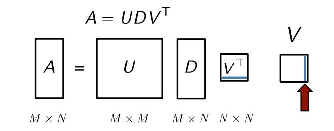
행렬 는 orthogonal matrix이고, 행렬 는 diagonal entries가 내림차순으로 정렬된 diagonal matrix입니다.
행렬 는 앞서 다룬 행렬 의 각 singular values에 해당하는 singular vector를 row형태로 나열한 것이며, 이를 행렬 로 transpose해서 살펴보면,
행렬 의 마지막 column은 가장 작은 singular value에 해당하는 singular vector임을 알 수 있습니다.
따라서 행렬 의 마지막 column이 을 풀기 위해 우리가 찾는 non-trivial solution이 됩니다. ( )
그렇지만, 마지막 column에 해당하는 singular value가 0이면 참 좋겠지만, 아닐 수도 있습니다. 그러나, 이 값이 인 조건 하에서 를 가장 최소화 하는 값을 나타낸다는 것은 변하지 않기 때문에 이 것을 해로 여깁니다.
Least Squares Problem
least squares 방법은 observation에 근거해 파라미터나 state를 추정하는 테크닉입니다.
state 를 predicted observation에 매핑시키기 위해 state 를 업데이트 해 나가는 과정입니다.
Predicted Observation이 real observation과 가깝도록 하는게 목표입니다.
많은 분야에서 사용됩니다. (Mapping, Localization, SLAM, Calibration, Bundle Adjustment...)
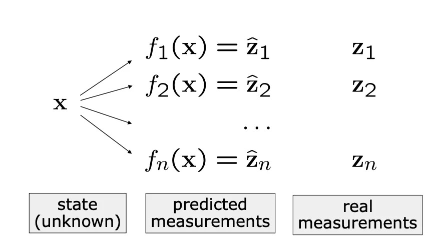
Predicted measurement와 real measurement 사이의 차를 최소화하는 방향으로 식을 전개하며
Sum of the Squared Error 형태로 나타나게 됩니다.
Error는 predicted 와 Actual measurement의 차이로 표현됩니다.
이 때, 이 Error는 평균이 0인 normal distribution의 분포를 가진다고 가정합니다.
이러한 분포를 표현하기 위해 information matrix 를 사용하며,
앞서 제시한 squared error of a measurement를 표현하면 아래와 같습니다.
참고로, squared error of a measurement의 결과는 scalar의 형태를 띄게 됩니다.
이러한, Error Function은 linear한 형태가 아니기 때문에, 선형화 하는 과정이 필요합니다.
이 때, Taylor Expansion을 이용합니다.
행렬 는 Jacobian을 의미합니다.
이후 Gauss-Newton 방식에 의해 다음과 같이 반복하여 해를 구합니다.
(1) state 근처에서 선형화 하기
(2) Linear System에 해당하는 term들 구하기
(3) Linear System을 풀기
이후 계속해서 state 를 로 업데이트 합니다.
가우스 뉴턴법 말고도 Levenberg-Marquadt 방법도 존재합니다.
이러한 non-linear least squares solving 하는 방법에 대해서는 따로 지면을 할애해 서술해 보겠습니다!
Skew-symmetric Matrix
skew-symmetric matrix는 를 만족하는 행렬 를 말합니다.
이러한 행렬은 main diagonal이 0의 값을 가지고 을 만족합니다.
주로 이러한 skew-symmetric matrix를 통해 cross-product를 표현할 때 많이 사용합니다.
Derivative of a Rotation Matrix
앞서 다룬 skew-symmetric matrix를 이용해 Rotation Matrix의 derivative를 구할 수 있습니다.
아래 과정은 유도하는 과정을 나타낸 것입니다.
임의의 rotation matrix 에 대해서, 가 성립된다는 것을 알고 있습니다.
x축을 기준으로 만큼 회전하는 rotation matrix 를 생각해봅니다. 를 만족합니다.
위의 식에서 양변을 에 대하여 미분해보면,
곱미분 성질을 이용하여 아래와 같이 서술할 수 있습니다.
성질을 이용하면,
와 같이 표현할 수 있고, 로 치환하게 되면,
행렬 는 를 만족하는 skew-symmetric matrix임을 알 수 있습니다.
주어진 행렬 를 실제 rotation matrix 를 이용해 구해보면,
이는 x축에 대한 unit vector 를 이용한 skew-symmetric matrix 로 표현 가능합니다.
따라서 아래와 같이 서술 할 수 있으며,
양변에 를 곱하게 되면,
정리하면, rotation matrix 의 derivative는 skew-symmetric matrix 와 rotation matrix 의 곱의 형태로 표현할 수 있습니다.
x축 말고도 임의의 다른 축 에 대해서도 적용됩니다.

