
3차원 월드 좌표계의 한 점에서 카메라 2차원 센서 좌표계의 한 점으로 어떻게 매핑되는지 묘사해보자!
2D pixel coordinate() ← 3D world coordinate()
Coordinate System의 종류
1.
World / object coordinate system (index가 없다는 건 object sys를 의미한다)
2.
Camera Coordinate System
3.
Image Plane Coordinate System
4.
Sensor Coordinate System
우리는 이제 system들간의 변환 관계에 대해서 살펴보게 될 것이다.
아래는 변환 과정을 시각적으로 묘사한 그림이다.
Transformation
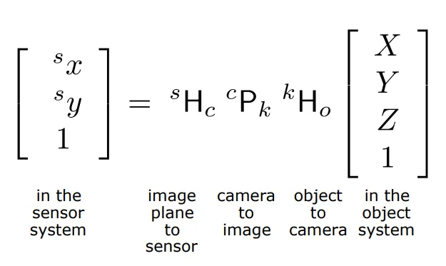

변환과정은 크게 4가지 단계로 나뉘어진다.
[1단계] Rigid body Transformation(World → Camera)
Extrinsic Parameters

카메라가 world 좌표계에서 어떤 위치와 방향(Pose)을 가지는 지를 설명하는 파라미터입니다.
•
총 6개의 파라미터가 필요합니다! (position : 3개 / Heading : 3개)
•
Invertible합니다!
Transformation
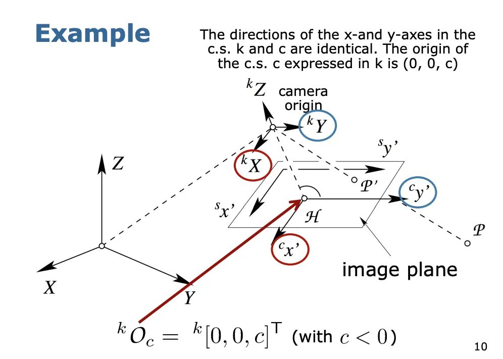
world coordinate 상의 점 를 아래와 같이 정의한다.
카메라 coordinate의 원점 O를 아래와 같이 정의한다.
변환을 위해서는 Translation과 Rotation이 수반되고 이를 반영하는 식은 아래와 같다.
이것은 Euclidian coordinates에서 표현하는 방식이 된다.
Homogenous coordinates에서 표현해보면 아래와 같다.
따라서, world coordinates에서 카메라 coordinates으로 변환하는 행렬이 완성되었다.
[2단계] Central Projection(Camera → Image)
Intrinsic Parameters
카메라 좌표계의 점에서 센서 좌표계의 점까지 투영하는 과정에서의 파라미터를 말하며, 카메라 앞의 scene과 이미지 평면 픽셀 간의 매핑을 나타냅니다.
•
Central Projection의 경우 Invertible하지 않지만,
Image to Sensor, Model Deviation은 invertible합니다.
Ideal Perspective Projection
•
무왜곡 렌즈이다
•
모든 광선은 곧은 직선의 형태로 나타내며 Projection center를 통과한다. 이 점은 카메라 좌표계의 원점 이다.
•
Focal point와 principal point 가 optical axis(가로축)에 놓여 있다.
•
카메라 원점과 이미지 평면과의 거리를 로 표현한다. (주로 < 0 으로 둔다, 그대로 두면 상이 반대로 맺히기 때문입니다)
(Projection center 와 principal Point 의 거리 = focal length)
여기서 삼각형의 닮음 관계를 이용하여 이미지 평면에 투영된 점 를 얻게 된다.
Homogenous Coordinate에서 표현한다면
최종적인 world 좌표계에서 이미지 평면까지의 앞서 구한대로 변환 결과가 도출된다.
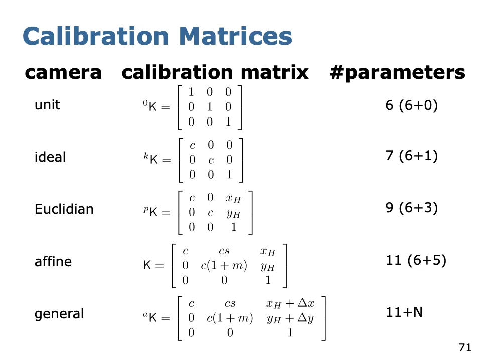
Calibration Matrix
위의 결과를 기호로 모델링한다면 아래와 같다.
이런 상황에서 각 기호들을 묶어 조금 더 보기 직관적이게 표현한다면
이 때, 우리는 새로운 이상적인 카메라 라는 가정하에 Calibration Matrix를 정의할 수 있다. (단, 이 경우는 ideal camera를 한정한다)
이 matrix를 이용해서 우리는 전체적인 mapping을 아래와 같이 표현 할 수 있다.
따라서 우리는 world 좌표계의 한 점으로부터 이미지 평면으로 투영되는 점을 구하게 된다.
위 식을 행렬 꼴로 풀면 아래와 같다.
마지막으로 실제 값을 구하기 위해 Euclidian Coordinates에서 표현하면 마무리 된다!
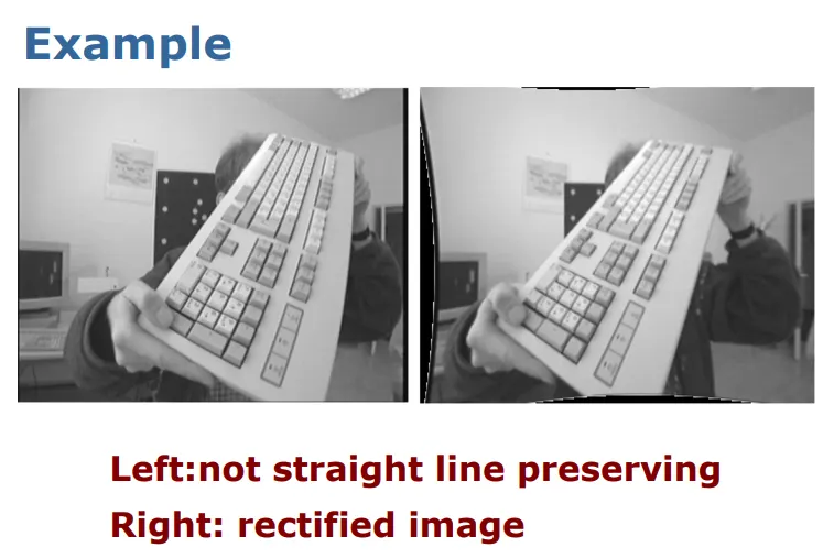
[3단계] Affine Transformation (Image → Sensor)
•
linear error만을 고려합니다, Non-linear Error는 고려하지 않습니다.
•
pixel coordinate로의 mapping이라고 부르기도 합니다.
Location of the Principal Point
sensor system의 원점이 image plane에서의 Principal point에 존재하지 않기 때문에
shift를 통해서 옮겨주어야 합니다.
Shear and Scale Difference
x와 y 사이의 Scale difference 과 Shear compensation s를 추가해줍니다.
(디지털 카메라에 한해서는 일반적으로 으로 간주할 수 있습니다)
여기까지 구하면 우린 이제 Sensor 평면에서의 좌표를 얻을 수 있습니다!
Calibration Matrix
변환 는 Calibration matrix 와 결합하여 새로운 Calibration Matrix를 만듭니다.
이 Calibration matrix가 affine transformation 그 자체입니다.
정리하면, affine transformation은 5가지 파라미터를 포함합니다.
•
Camera constant:
•
principal point:
•
scale difference:
•
shear:
DLT : Direct Linear Transform (지금까지의 여정을 다 합치는 변환)
Object coordinate system에서부터 Sensor coordinate system까지의 변환과정을 의미한다.
affine camera를 모델링 한 것입니다.
이 과정에서 우리는 총 11개의 파라미터를 얻게 된다.
extrinsic parameters: (6개), intrinsic parameters: (5개) → 총 11개!
Homogeneous coordinate이 아닌 Euclidian space에서의 좌표를 표현하면 아래와 같다.
[4단계] Non-linear Error Correction (In Sensor)
•
이 단계에서 이전에 고려하지 않았던 non-linear error를 보정합니다!
•
non-linear error가 생기는 이유는 무엇일까요? → (1) 부정확한 렌즈 (2) 센서의 평면성 등등......
General Mapping
따라서 전체적인 mapping은 다음과 같다.
이렇게 non-linear errors까지 보정을 하고 나면 아래와 같은 결과를 얻을 수 있다.
General Calibration Matrix
General Calibration Matrix는 하나의 affine camera와 general mapping을 결합 한다.
따라서 최종적인 general camera model이 완성된다 (진짜 끝판대장)
distortion은 따로 포스트를 할애해 작성해 보도록 하겠습니다.
카메라 분류하기
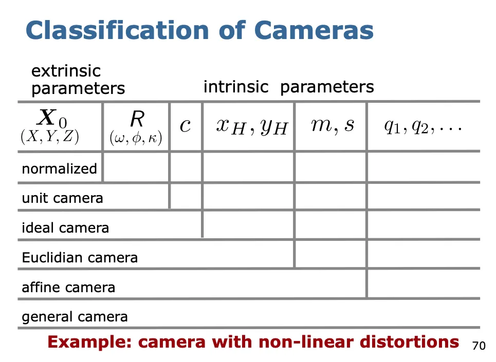
Calibrated Camera 정의하기
•
intrinsic 파라미터를 모른다면, 우리는 카메라가 uncalibrated 되었다고 부릅니다.
•
intrinsic 파라미터를 안다면, 우리는 카메라가 calibrated 되었다고 부릅니다.
•
intrinsic 파라미터를 얻는 과정이 바로 camera calibration입니다.
•
만약 intrinsic 파라미터를 알고 그 값이 변하지 않는다면, 우리는 이러한 카메라를 metric camera라고 부릅니다.
