Inner Product
벡터 가 주어졌을 때 각 벡터는 행렬로 생각할 수 있고, 는 행렬로 생각할 수 있다.
를 inner product 혹은 dot product 로 정의하며 로 표기한다.
inner product는 아래와 같은 성질을 만족한다. (는 벡터, 는 스칼라)
또한 inner product는 각 벡터의 norm과 angle을 이용해 표현할 수도 있다.
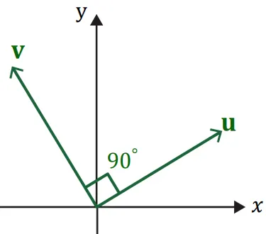
이 때, 만약 을 만족한다면 서로 orthogonal 하다고 한다.
를 만족하기 때문에 내적값이 0이 된 것이며 벡터 는 서로 수직이다.
Vector Norm
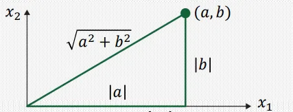
에 대하여, length (혹은 norm)은 의 제곱근으로 정의되며, 양수의 스칼라값으로 정의된다.
이러한 norm은 기하학적으로 원점으로부터 까지를 잇는 선의 길이를 의미한다.
또한 임의의 scalar 값 에 대해, 의 length는 의 길이에 만큼 곱한 값이다.
참고로, length가 1인 벡터를 unit vector 라고 한다.
vector를 normalize 한다는 뜻은, 벡터 가 주어졌을 때, 그것의 length로 나누어주는 것을말한다.
는 와 같은 방향을 가리키며, 길이만 다르게 된다. (의 length는 1)
Distance between Vectors in
벡터 에 대해 distance between 는 아래와 같이 정의됩니다.
Least Squares 문제
변수의 개수() 보다 방정식의 개수()가 더 많은 경우, Over-determined Linear System이다.
일반적으로 이러한 경우는 해가 없다. 하지만 우리는 근사적이라도 값을 구하고 싶다!
Overdetermined system 에 대하여, ()
이러한 시스템의 해 는 아래 와 같이 정의 된다.
어떤 를 선택하더라도, 벡터 는 의 영역 안에 존재하게 될 것이다.
따라서, 우린 벡터 와 가장 가깝게 위치하는 위의 한 점을 찾는것, 그 때의 를 찾는것이 목표이다.
위의 설명을 그림으로 표현하면 아래와 같다.
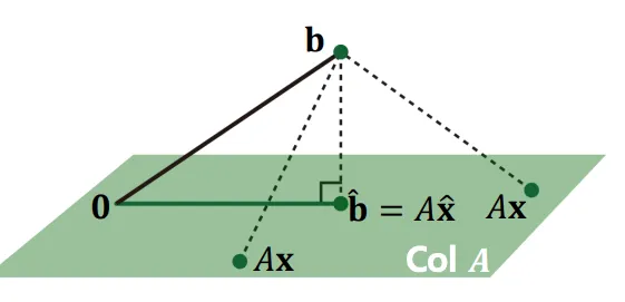
이 때, 점 은 에 존재하는 점 중 점 와 가장 가까운 점이다.
이러한 조건 하에서 벡터 는 와 반드시 orthogonal 하게 된다.
여기서 벡터 은 를 구성하는 basis 벡터를 말한다.
이와 동일하게 서술하면,
따라서 least squres problem을 푸는 식이 완성된다.
Normal Equation
앞서 제시한 Least Squares Problem을 푸는 방법 중 하나가 바로 normal equation입니다.
주어진 least square problem 의 식을 풀기 위해 정답에 가장 가까운 해를 구할 것 입니다.
해를 구하기 위해 사용하는 식이 위에 제시한 normal equation 입니다.
이러한 형태는 새로운 Linear System 의 꼴로 표현할 수 있습니다.
만약 가 invertible 하다면, 그 해는 아래와 같이 구해질 수 있다.
따라서 앞서 주어진 그림을 살펴보았을 때,
점 에서 로의 orthogonal projection 과정을 아래와 같이 나타낼 수 있다.
만약 가 invertible 하지 않다면?
•
가 invertible 하지 않기 위해서는 행렬 가 Linearly dependent 해야한다.
(즉, lineary dependent하면 invertible 하다)
•
이러한 경우 해는 항상 무수히 많은 경우가 된다! (→ 해가 없는 경우는 사실상 존재하지 않는다)
•
일반적으로, 현실 데이터셋을 다룰 때 invertible 하지 않은 경우는 없다! (거의 95% 이상)
데이터셋이 많아지면 많아질 수록 feature 간에 linearly dependent한 경우가 높은 확률로 사라지기 때문이다.
Orthogonal and Orthonormal Sets
벡터의 집합 에 대햐여, 각 벡터쌍들이 를 만족하면 orthogonal set이라고 정의한다.
벡터의 집합 에 대하여, orthogonal set이라고 가정했을 때, 각 벡터들이 unit vector이다면, orthonormal set이라고 정의한다.
벡터들이 Orthogonal하다면 linearly independent하다고 볼수 있지만,
벡터들이 linearly independent하다고 해서 Orthogonal 하다고 할수 없다.
Orthogonal Projection of
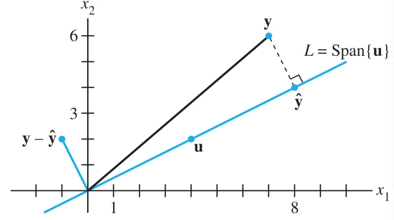
(1) line에 projection하기
one-dimensional subspace 에 projection을 한다면 아래와 같은 식으로 표현 가능하다
만약, 벡터 가 unit vector라면, 아래와 같이 표현할 수도 있다.
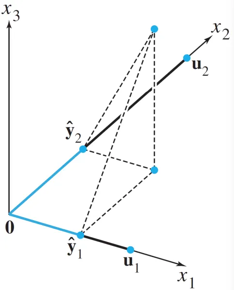
(2) Plane에 projection하기
two-dimensional subspace 에 projection 한다면 아래와 같이 표현한다.
만약, 벡터 가 unit vector라면, 아래와 같이 표현할 수도 있다.
Transformation: Orthogonal Projection
위에 제시한 orthogonal projection 과정을 식으로 표현하면,
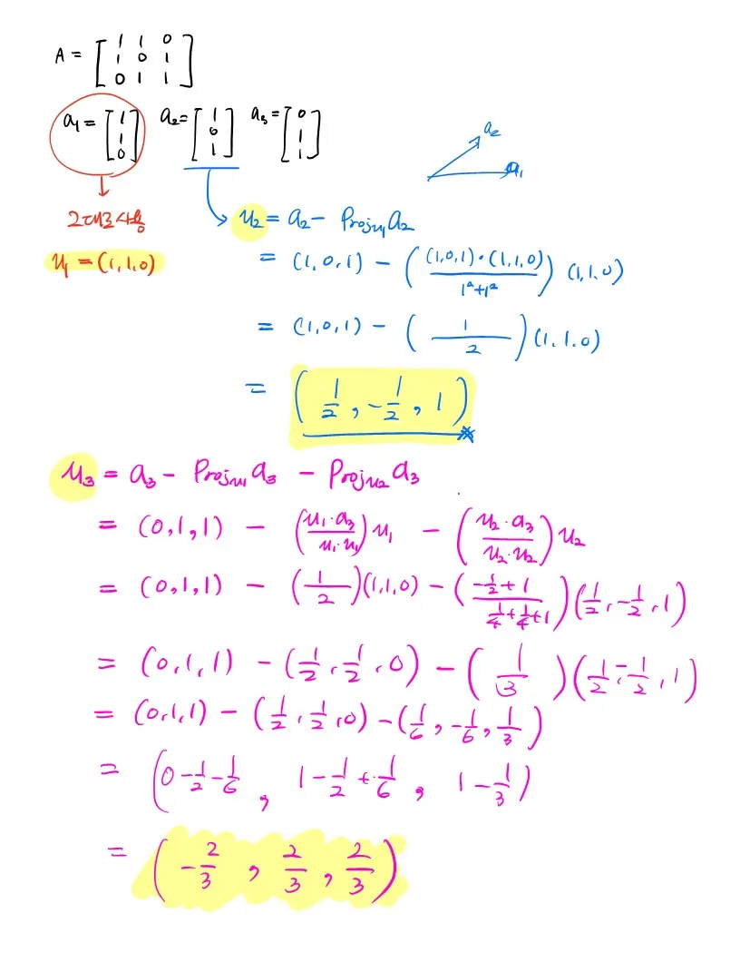
Gram-Schmidt Orthogonalization
이 방법은 상의 subspace에서 orthogonal 하거나 orthonormal한 basis를 만들기 위해 사용되는 단순한 알고리즘입니다.
하는 상황을 가정하였을 때, 이다.
이러한 상황에서 subspace 에서의 orthogonal basis를 만들기 위해 사용한다.
이라고 가정한 뒤, 를 에 orthogonal한 벡터라고 생각한다면, 아래 식과 같이 표현할 수 있다.
실제로 를 행해보면 값이 0이 나온다는 것을 알 수있다.
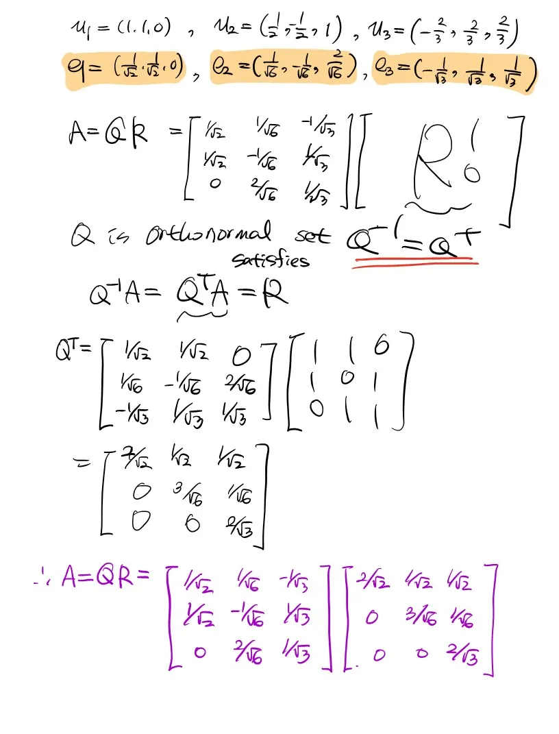
QR Factorization
위에서 언급한 Gram-Schmidt 방법을 이용해 orthonormal vector를 구했는데, 이를 이용해 행렬을 분해하는 방법이 QR Factorization (= QR decomposition)이다. 수학적인 정의는 아래와 같다.
행렬 가 의 크기를 갖는 행렬로 주어지고,
각 column들이 linearly independent하다고 가정하면,
의 형태로 표현할 수 있다. 는 크기의 행렬이고,
각 column들은 를 구성하는 orthonormal basis이다.
은 크기의 upper trinangular 형태를 가지는 행렬이며, 역행렬이 존재한다.
분해하는 과정을 짧게 나마 서술해보면.
1.
주어진 행렬의 column vector들을 나눠놓은 후 각각 Gram-Schmidt 방법을 적용시킨다.
2.
orthogonalize 된 벡터들을 normalize 하기 위해 각각의 norm으로 나눠준다 (크기를 1로 만듬= 정규화)
3.
이 벡터들을 순서대로 모으면 행렬 가 되고, 이 행렬은 orthonormal 하다.
4.
orthonormal 행렬의 성질 을 이용해 를 유도할 수 있습니다. 이를 이용해 행렬 을 구하면 factorization이 끝난다.
아래 풀이는 임의로 주어진 행렬에 대해 QR decomosition을 해보는 예제이다.