EVD와 SVD의 차이
Eigenvalue Decomposition의 경우 square matrix를 대상으로 하는 반면에,
Singular Value Decomposition은 크기의 rectangular matrix를 대상으로 한다.
일반적으로 SVD의 경우 크기의 행렬 를 하여 square matrix 형태로 만든후 EVD를 실행하는 것이다.
Algebraic/Geometric Multiplicity
앞선 포스트를 통해 n개의 linearly independent한 eigenvector가 존재한다면 Diagonalizable하다는 것을 배웠다. 그렇다면 어떤 상황에서 n개의 linearly independent한 eigenvector를 뽑을 수 있을까?
일반적으로 를 진행하여 나올수 있는 근의 전체 개수는 행렬 A의 column 개수 n개이다.
하지만 (1) n개중 에서 허근이 있다면? n개의 linearly independent한 eigenvector를 뽑을 수 없게 된다.
또한 중근이 존재한다면 그 eigenvalue에 해당하는 eigenvector가 2개 나올 수 있으며, 만약 (2) 이 두 개가 Linearly dependent한 경우에도 n개의 linearly independent한 eigenvector를 뽑을 수 없다.
Algebraic Multiplicity는 특성방정식으로 표현할 때 나오는 중근의 개수를 말하고,
Geometric Multiplicity는 동일한 에 대하여 linearly independent한 eigenvector의 개수를 말한다.
예를 들어, 라는 특성 방정식이 주어졌을 때 각 eigenvalue에 대한 multiplicity를 표로 정리하면 아래와 같다.
비교 | lambda = 0 | lambda = -5 |
A.M | 2 | 1 |
G.M | 2여야 함! | 1 |
이 때, A.M > G.M 인 경우, 전체 가질 수 있는 eigenvector의 개수를 충족하지 못하므로, eigendecomposition이 불가능 해진다.
The Spectral Theorem
symmetric matrix인 행렬 가 주어졌을 때, 아래 성질을 가집니다!
•
행렬 는 개의 실수 eigenvalue를 가집니다.(multiplicity 고려해서)
•
각 eigenvalue 에 대한 eigenspace의 dimension은 특성 방정식에서의 근 의 multiplicity와 같습니다.
(Geometric Multiplicity == Algebraic Multiplicity)
•
각 에 해당하는 eigenspace는 서로 orthogonal합니다.
즉, eigenvalue가 다른 eigenvector들은 서로 orthogonal 합니다.
•
위의 성질을 만족하는 행렬 는 orthogonally diagonalizable 합니다.
Orthogonal Matrix란?
아래 두 조건을 만족하는 행렬을 말한다.
•
행렬을 구성하는 row vector 혹은 column vector의 길이가 1이다.
•
각 row vector 또는 column vector들이 서로 수직이다.
위 조건을 통해 아래 수식을 만족하게 되고, 이를 통해 쉽게 역행렬을 구할 수 있습니다.
이러한 Orthogonal matrix의 성질에는 크게 4가지가 존재합니다.
•
Orthogonal Matrix를 Transpose 해도 Orthogonal Matrix 입니다.
•
Orthogonal Matrix의 역행렬 또한 Orthogonal Matrix 입니다.
•
Orthogonal Matrix 끼리의 곱의 결과도 Orthogonal Matrix입니다.
•
Orthogonal Matrix의 Determinent는 1 또는 -1입니다.
Orthogonally Diagonalizable하다는 것의 의미?
말 그대로 orthogonal한 성질을 가지면서 diagonalize를 할 수 있다는 것이다.
•
diagonalizable ⇒ eigen decomposition이 가능하다.
•
orthogonal ⇒ distinct한 eigenvalue에 대해서는 eigenvector가 orthogonal합니다.
그러나 같은 eigenvalue에 해당하는 eigenvector끼리는 orthogonal하지 않을 수 있는데,
이를 위해 QR-decomposition을 활용해 서로 orthogonal하게 만든다.
Quadratic Form의 변수 변경하기
Quadratic form은 공간상의 함수 를 말하며, 아래의 식으로 표현될 때 정의할 수 있다.
이 때 행렬 는 symmetric matrix이다.
이러한 Quadratic form을 이용해서 임의의 식으로 주어졌을 때, 행렬의 곱의 형태로 표현 가능하다.
이러한 Quadratic form에는 중요한 성질이 있는데, 아래와 같다.
행렬 가 symmetric matrix라고 가정하였을 때, 변수 를 orthogonal changing 한다.
이러한 변환은 quadratic form 로 하여금 의 형태로 바뀌게 하며, 행렬 는 cross-product term이 없고 행렬 의 eigenvalue로만 이루어진 diagonal matrix이다.
이 때, 행렬 의 column들은 의 quadratic form의 principal axes라고 불리운다.
식으로 유도한다면, 와 같이 표현되며,
행렬 가 symmetric 하기 때문에, 를 만족시키는 eigenvalue로 이루어진 행렬 가 반드시 존재한다.
이런 변환을 함으로써 어떠한 quadratic form으로 주어져도 cross-product이 없는 형태의 quadratic form으로 바꿀 수 있다. (변환의 가장 큰 이유!!!)
이러한 변환을 기하학점 관점에서 살펴보면 다음과 같다.
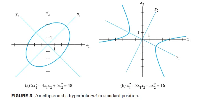
3-(a)의 경우를 보면 의 식을 변환을 하게 되면,
의 꼴로 바뀌며,
바꾸는데 사용한 행렬 의 column들이 새로운 좌표계의 basis vector가 됨을 알 수 있다!
Quadratic Form 분류하기
Quadratic form 는 아래 3가지로 분류한다.
•
positive definite
•
negative definite
•
indefinite
0을 포함하는 경우, positive semi-definite,
negative semi-definite 라고 정의한다.
위와 같은 분류를 eigenvalue와의 연관성을 고려한다면 아래와 같이 서술 할 수 있다!
행렬 가 symmetric matrix라고 가정하였을 때, quadratic form 는
•
positive definite하다는 것은 행렬 의 eigenvalue들이 모두 양수이다는 것과 동치이다.
•
negative definite하다는 것은 행렬 의 eigenvalue들이 모두 음수이다는 것과 동치이다.
•
indefinite하다는 것은 행렬 의 eigenvalue들이 양수 또는 음수로 이루어져있다는 것과 동치이다.
Constrained Optimization
행렬 가 symmetric matrix라고 가정하고, 값 을 아래와 같이 정의할 때
은 행렬 의 가장 작은 eigenvalue와 같고, 이 때의 는 그에 해당하는 eigenvector일 때이다. 반대로, 은 행렬 의 가장 큰 eigenvalue와 같고, 이 때의 는 그에 해당하는 eigenvector일 때이다.
→ svd로 해를 구할 때 사용 (를 풀 때 사용)